728x90
Ridge, Lasso, Elastic Net
- Ridge
- 계수 정규화(Regularization)
- 전체 변수를 모두 유지하면서 각 변수의 계수 크기를 조정
- 종속변수 예측에 영향을 거의 미치지 않는 변수는 0에 가까운 가중치를 주게 하여 독립변수들의 영향력을 조정
- 위의 과정을 통해 다중공선성을 방지하면서 모델의 설명력을 최대화 ※다중공선성: 독립변수들사이의 관계가 깊어서 종속변수의 특징이 잘 안보임
- L2-norm
- 매개변수 alpha의 값을 조정하여 정규화 수준을 조정
- alpha 값이 0이면 선형회귀와 동일
- 값이 클수록 독립변수들의 영향력이 작아져 회귀선이 평균을 지나는 수평선이 됨
- 계수 정규화(Regularization)
- Lasso
- Ridge와 유사하지만 중요한 몇 개의 변수만 선택하고 나머지 변수들은 계수를 0으로 주어 변수의 영향력을 아예 없애는 점이 차이점
- 따라서 모델을 단순하게 만들 수 있고 해석이 용이
- L1-norm
- 매개변수 alpha의 값을 조정하여 정규화의 강도를 조정
- Ridge와 유사하지만 중요한 몇 개의 변수만 선택하고 나머지 변수들은 계수를 0으로 주어 변수의 영향력을 아예 없애는 점이 차이점
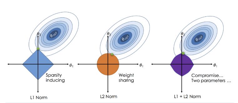
- Elastic Net
- Ridge와 Lasso의 최적화 지점이 다르기 때문에 두 정규화 항을 결합하여 절충한 모델
- Ridge는 변환된 계수가 0이 될 수 없지만 Lasso는 0이 될 수 있다는 특성을 결합
- Ridge와 Lasso의 혼합비율을 조절하여 성능을 최적화
- 혼합 비율이 0에 가까울수록 Ridge와 같아짐
- 혼합 비율이 1에 가까울수록 Lasso와 같아짐
- 독립변수를 이미 잘 정제해서 중요할 것으로 판단되는 변수들만 잘 선별해둔 상태라면
- Ridge와 Lasso의 최적화 지점이 다르기 때문에 두 정규화 항을 결합하여 절충한 모델
Ridge의 비율을 높이는 것이 유리하고, 변수 선택없이 주어진 독립변수를 모두 사용하는 형태라면 Lasso의 비율을 높이는 것이 유리
01. P-value 와 R-square 값에 따른 회귀모델 튜닝
- R-square가 높고 P-value가 0.05미만인 경우
- 통계적으로 의미가 있으며, 모델 설명력이 높음
- 이상적인 모형
- 주요 인자 추출
- 통계적으로 의미가 있으며, 모델 설명력이 높음
- R-square가 낮고 P-value가 0.05 미만인 경우
- 통계적으로 의미가 있으나, 모델 설명력이 낮음
- 이상치 제거
- 비선형 회귀분석 적용
- 데이터 확보(컬럼)
- 통계적으로 의미가 있으나, 모델 설명력이 낮음
- R-square가 높고 P-value가 0.05보다 높은 경우
- 통계적으로 의미가 없으나, 모델 설명력이 높음
- 데이터 확보(행)
- 이상치 제거
- 통계적으로 의미가 없으나, 모델 설명력이 높음
- R-square가 낮고 P-value 가 0.05보다 높은 경우
- 통계적으로 의미가 없으며, 모델 설명력이 낮음
- 새로운 변수 탐색
- 비선형 회귀분석 적용
- 통계적으로 의미가 없으며, 모델 설명력이 낮음
import pandas as pd
import numpy as np
from sklearn.linear_model import LinearRegression, Ridge, Lasso, ElasticNet
from sklearn.model_selection import train_test_split
import statsmodels.api as sm # 통계 모델링을 해줌 p-value같은 통계값을 확인시켜줌
import seaborn as sns
import matplotlib.pyplot as plt
from sklearn.preprocessing import PolynomialFeatures
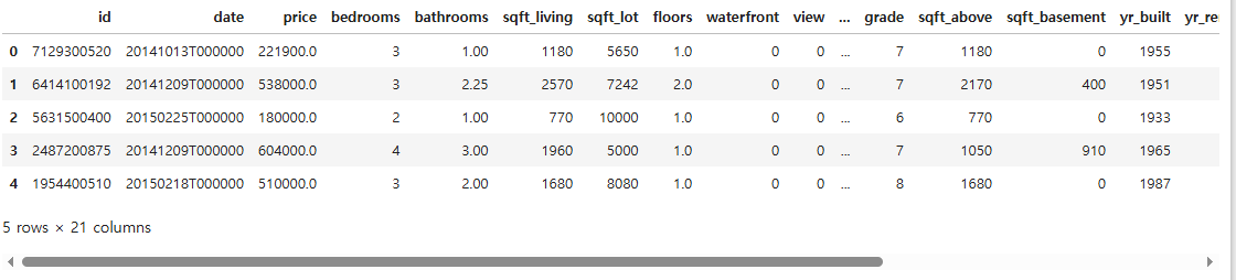
df = pd.read_csv("./data/kc_house_data.csv")
df.head()
df.columns
Index(['id', 'date', 'price', 'bedrooms', 'bathrooms', 'sqft_living',
       'sqft_lot', 'floors', 'waterfront', 'view', 'condition', 'grade',
       'sqft_above', 'sqft_basement', 'yr_built', 'yr_renovated', 'zipcode',
       'lat', 'long', 'sqft_living15', 'sqft_lot15'],
      dtype='object')
df.shape
(21613, 21)
df.info()
<class 'pandas.core.frame.DataFrame'>
RangeIndex: 21613 entries, 0 to 21612
Data columns (total 21 columns):
 #   Column         Non-Null Count  Dtype
---  ------         --------------  -----
 0   id             21613 non-null  int64
 1   date           21613 non-null  object
 2   price          21613 non-null  float64
 3   bedrooms       21613 non-null  int64
 4   bathrooms      21613 non-null  float64
 5   sqft_living    21613 non-null  int64
 6   sqft_lot       21613 non-null  int64
 7   floors         21613 non-null  float64
 8   waterfront     21613 non-null  int64
 9   view           21613 non-null  int64
 10  condition      21613 non-null  int64
 11  grade          21613 non-null  int64
 12  sqft_above     21613 non-null  int64
 13  sqft_basement  21613 non-null  int64
 14  yr_built       21613 non-null  int64
 15  yr_renovated   21613 non-null  int64
 16  zipcode        21613 non-null  int64
 17  lat            21613 non-null  float64
 18  long           21613 non-null  float64
 19  sqft_living15  21613 non-null  int64
 20  sqft_lot15     21613 non-null  int64
dtypes: float64(5), int64(15), object(1)
memory usage: 3.5+ MB
df.describe()
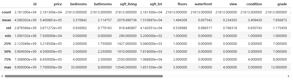
- bedrooms의 최댓값이 33인데 잘못된 값은 아닌지 확인이 필요함
df[["price", "sqft_living", "sqft_basement", "yr_built", "zipcode"]].corr()

# 데이터 시각화 하여 분포 확인
sns.pairplot(df[["price", "sqft_living", "sqft_basement", "yr_built", "zipcode"]])
plt.show()
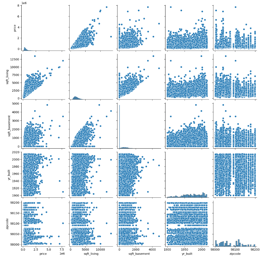
- price는 sqft_living과 강한 영향을 받을 것으로 추측
- yr_built 와도 약간의 관계가 있는 것으로 보임
- 최근에 지어진 집 중에 가격이 높은 경우가 있음
- sqft_living 과 sqft_basement 두 변수 간에 관계가 있음
- 독립변수 간의 상관성이 높으면 다중공선성을 유발하여 모델 성능을 저하시킬 수 있으므로 주의해야함
df.columns
Index(['id', 'date', 'price', 'bedrooms', 'bathrooms', 'sqft_living',
       'sqft_lot', 'floors', 'waterfront', 'view', 'condition', 'grade',
       'sqft_above', 'sqft_basement', 'yr_built', 'yr_renovated', 'zipcode',
       'lat', 'long', 'sqft_living15', 'sqft_lot15'],
      dtype='object')
# id, date는 키값에 해당하므로 변수에서 제외
x = df.drop(["id", "date", "price"], axis = 1)
y = df["price"]
x_train, x_test, y_train, y_test = train_test_split(x, y, test_size = 0.3, random_state = 25)
print(x_train.shape, x_test.shape)
(15129, 18) (6484, 18)
# 선형 회귀 모델 생성
lr = LinearRegression()
lr.fit(x_train, y_train)
# 테스트셋 예측
y_predict = lr.predict(x_test)
print(lr.score(x_train, y_train))
print(lr.score(x_test, y_test))
0.7026590431940445
0.6920828242645156
print(lr.coef_, lr.intercept_)
[-3.61945247e+04  4.25337124e+04  1.11252551e+02  1.20894087e-01
  8.25811374e+03  6.09380415e+05  5.83343473e+04  2.68761614e+04
  9.27427943e+04  6.93491604e+01  4.19033908e+01 -2.62504750e+03
  2.16620394e+01 -5.91515914e+02  6.07818249e+05 -2.08265478e+05
  2.21473821e+01 -3.60683954e-01] 8157651.179475979
# 자세한 모델 결과값을 확인하고 싶을 때는 OLS(Ordinary Least Squares) 패키지를 사용
ols_m = sm.OLS(y_train, sm.add_constant(x_train)).fit()
# sm에는 stats모델이 없기 때문에 상수항을 추가(add_constant)/ fit():훈련
ols_m.summary()

# const coef 교차되는 값: y절편
# P > |t| 값이 0.05이하로 나오는 값이 있으면 통계적으로 유의미하다
# PolynomialFeatures
# 변수 변환
poly_m = PolynomialFeatures(include_bias = False)
x_train_poly = poly_m.fit_transform(x_train)
x_test_poly = poly_m.transform(x_test)
x_train_poly.shape
(15129, 189)
x_train.shape # 컬럼이 189개 까지 늘어남
(15129, 18)
lr_poly = LinearRegression()
lr_poly.fit(x_train_poly, y_train)

print(lr_poly.coef_, lr_poly.intercept_)
[ 1.47365252e+07 -7.11958184e+06 -1.33894934e+04 -3.08151209e+02
 -4.11004271e+07  9.44333725e+07  8.35340794e+06 -1.57709072e+06
 -1.84845254e+07  3.67372844e+04 -2.51294940e+04  2.00304092e+04
  2.85479629e+04 -5.35851027e+05  1.10401356e+08  6.54511443e+06
  ...
print(lr_poly.score(x_train_poly, y_train))
print(lr_poly.score(x_test_poly, y_test))
0.8313639205138337
0.7998005316961556
# Ridge
# alpha 별 모델 생성
ridge = Ridge(alpha = 1)
ridge001 = Ridge(alpha = 0.01)
ridge100 = Ridge(alpha = 100)
ridge.fit(x_train_poly, y_train)
ridge001.fit(x_train_poly, y_train)
ridge100.fit(x_train_poly, y_train)

# 모델 별 R-Square 산출
print("ridge R2")
print(ridge.score(x_train_poly, y_train))
print(ridge.score(x_test_poly, y_test))
print("ridge001 R2")
print(ridge001.score(x_train_poly, y_train))
print(ridge001.score(x_test_poly, y_test))
print("ridge100 R2")
print(ridge100.score(x_train_poly, y_train))
print(ridge100.score(x_test_poly, y_test))
ridge R2
0.8322834997317592
0.8016302187568957
ridge001 R2
0.8337567538023641
0.8037555055389426
ridge100 R2
0.8175836696179786
0.7862830838590333- alpha값을 100으로 설정할 경우 과소적합으로 인해 성능이 떨어짐
# Lasso
# alpha 별 모델 생성
lasso = Lasso(alpha = 1)
lasso001 = Lasso(alpha = 0.01)
lasso100 = Lasso(alpha = 100)
lasso.fit(x_train_poly, y_train)
lasso001.fit(x_train_poly, y_train)
lasso100.fit(x_train_poly, y_train)

# 모델 별 R-Square 산출
print("lasso R2")
print(lasso.score(x_train_poly, y_train))
print(lasso.score(x_test_poly, y_test))
print(np.sum(lasso.coef_ != 0))
print("lasso001 R2")
print(lasso001.score(x_train_poly, y_train))
print(lasso001.score(x_test_poly, y_test))
print(np.sum(lasso001.coef_ != 0))
print("lasso100 R2")
print(lasso100.score(x_train_poly, y_train))
print(lasso100.score(x_test_poly, y_test))
print(np.sum(lasso100.coef_ != 0))
lasso R2
0.7914192419092956
0.7589043565110895
189
lasso001 R2
0.7914203188310407
0.7589341680213767
189
lasso100 R2
0.7912671615690783
0.7594114127524878
175- ElasticNet 은 기본적으로 alpha와 l1_ratio 를 설정
- 여기서 alpha는 Ridge와 Lasso의 alpha와는 다름
- ElasticNet의 정규화는 Ridge와 Lasso를 합친 것이므로 alpha L1 + beta L2 임
- l1_ratio는 0에서 1의 값을 가지며 Lasso 모델의 비중을 나타냄
- l1_ratio가 1이면 Lasso와 같고 0이면 Ridge와 같은 모델이 됨
# 모델 생성
elast = ElasticNet()
elast01 = ElasticNet(l1_ratio = 0.1)
elast09 = ElasticNet(l1_ratio = 0.9)
elast.fit(x_train_poly, y_train)
elast01.fit(x_train_poly, y_train)
elast09.fit(x_train_poly, y_train)
# 모델 별 R-Square 산출
print("elast R2")
print(elast.score(x_train_poly, y_train))
print(elast.score(x_test_poly, y_test))
print(np.sum(elast.coef_ != 0))
print("elast01 R2")
print(elast01.score(x_train_poly, y_train))
print(elast01.score(x_test_poly, y_test))
print(np.sum(elast01.coef_ != 0))
print("elast09 R2")
print(elast09.score(x_train_poly, y_train))
print(elast09.score(x_test_poly, y_test))
print(np.sum(elast09.coef_ != 0))
elast R2
0.7896486877389272
0.7603804351036108
188
elast01 R2
0.7893596411326199
0.7606153418735575
189
elast09 R2
0.7902421336693677
0.7597645858593042
188
728x90
'08_ML(Machine_Learning)' 카테고리의 다른 글
| 14_로지스틱 회귀 (0) | 2025.04.07 |
|---|---|
| 12_야구선수 연봉_선형회귀 (1) | 2025.04.04 |
| 10_다중 선형 회귀 규제 (0) | 2025.04.04 |
| 09_선형 회귀 실습 (0) | 2025.04.04 |
| 08_선형회귀 (0) | 2025.04.04 |