728x90
프로 야구선수 연봉 예측
import pandas as pd
import numpy as np
import matplotlib.pyplot as plt
import seaborn as sns
from sklearn.preprocessing import StandardScaler, OneHotEncoder # 사이킷런에서도 원핫인코딩을 제공해줌
from sklearn.model_selection import train_test_split
from sklearn.linear_model import LinearRegression
from sklearn.metrics import mean_absolute_error
from statsmodels.stats.outliers_influence import variance_inflation_factor
import statsmodels.api as sm # 통계모델사용
# Windows용 한글 폰트 오류 해결
from matplotlib import font_manager, rc
font_path = "C:/Windows/Fonts/malgun.ttf"
font_name = font_manager.FontProperties(fname = font_path).get_name()
rc("font", family = font_name)
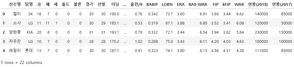
01. 데이터 확인
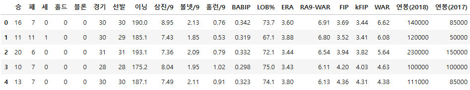
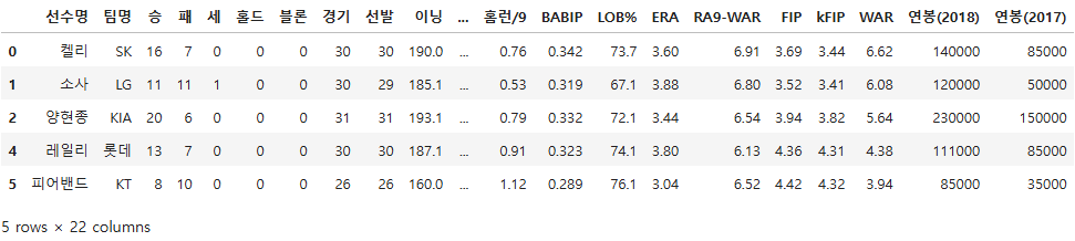
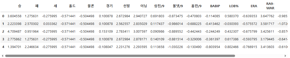
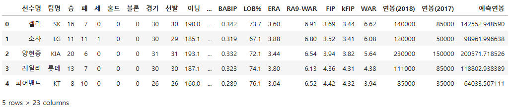
pich = pd.read_csv("./data/picher_stats_2017.csv")
pich.head()
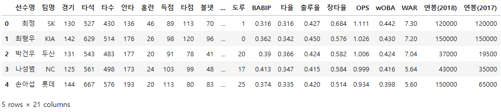
batt = pd.read_csv("./data/batter_stats_2017.csv")
batt.head()
pich.shape
(152, 22)
pich[pich["연봉(2018)"] != pich["연봉(2017)"]]
pich.info() # 계산하고자 하는 값들은 int64이므로 전처리 필요 없음
<class 'pandas.core.frame.DataFrame'>
RangeIndex: 152 entries, 0 to 151
Data columns (total 22 columns):
 #   Column    Non-Null Count  Dtype
---  ------    --------------  -----
 0   선수명       152 non-null    object
 1   팀명        152 non-null    object
 2   승         152 non-null    int64
 3   패         152 non-null    int64
 4   세         152 non-null    int64
 5   홀드        152 non-null    int64
 6   블론        152 non-null    int64
 7   경기        152 non-null    int64
 8   선발        152 non-null    int64
 9   이닝        152 non-null    float64
 10  삼진/9      152 non-null    float64
 11  볼넷/9      152 non-null    float64
 12  홈런/9      152 non-null    float64
 13  BABIP     152 non-null    float64
 14  LOB%      152 non-null    float64
 15  ERA       152 non-null    float64
 16  RA9-WAR   152 non-null    float64
 17  FIP       152 non-null    float64
 18  kFIP      152 non-null    float64
 19  WAR       152 non-null    float64
 20  연봉(2018)  152 non-null    int64
 21  연봉(2017)  152 non-null    int64
dtypes: float64(11), int64(9), object(2)
memory usage: 26.3+ KB
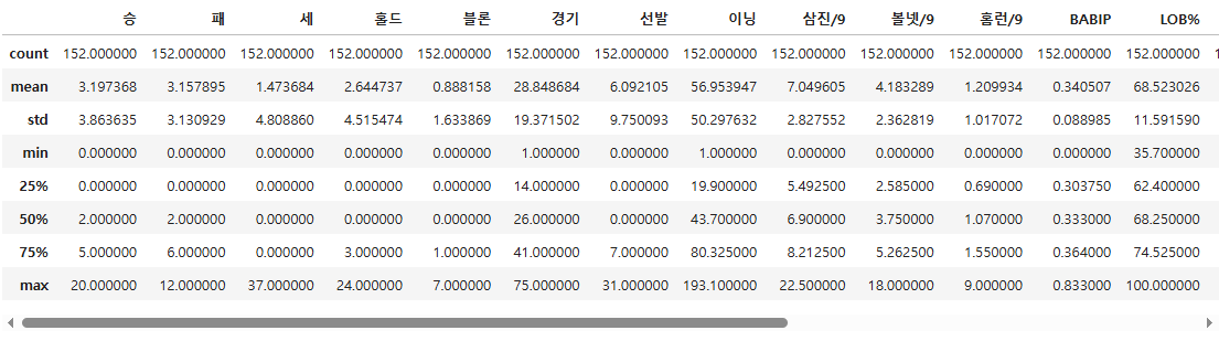
pich.describe()
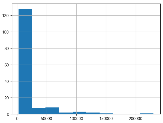
# 2018년 투수 연봉 분포 히스토그램
pich["연봉(2018)"].hist()
plt.show()
# 2018년 연봉의 상자 그림 출력
pich.boxplot(column = ["연봉(2018)"])
plt.show()

- 종속변수 분석
- 수십억의 연봉을 받는 프로야구선수는 많지 않으며, 5억원 미만의 연봉이 일반적임
# 선수명, 팀명과 같이 그래프로 표현할 수 없는 피처 제외하고 시각화
vis_pich = pich.iloc[:, 2:]
vis_pich.head()
# 피처 각각에 대한 히스토그램을 출력
def plot_hist(df):
fig = plt.figure(figsize = (20, 16))
# df의 열 수 만큼의 subplot을 출력
for i in range(len(df.columns)):
ax = fig.add_subplot(5, 5, i + 1)
plt.hist(df[df.columns[i]], bins = 50)
ax.set_title(df.columns[i])
plt.tight_layout()
plt.show()
plot_hist(vis_pich)
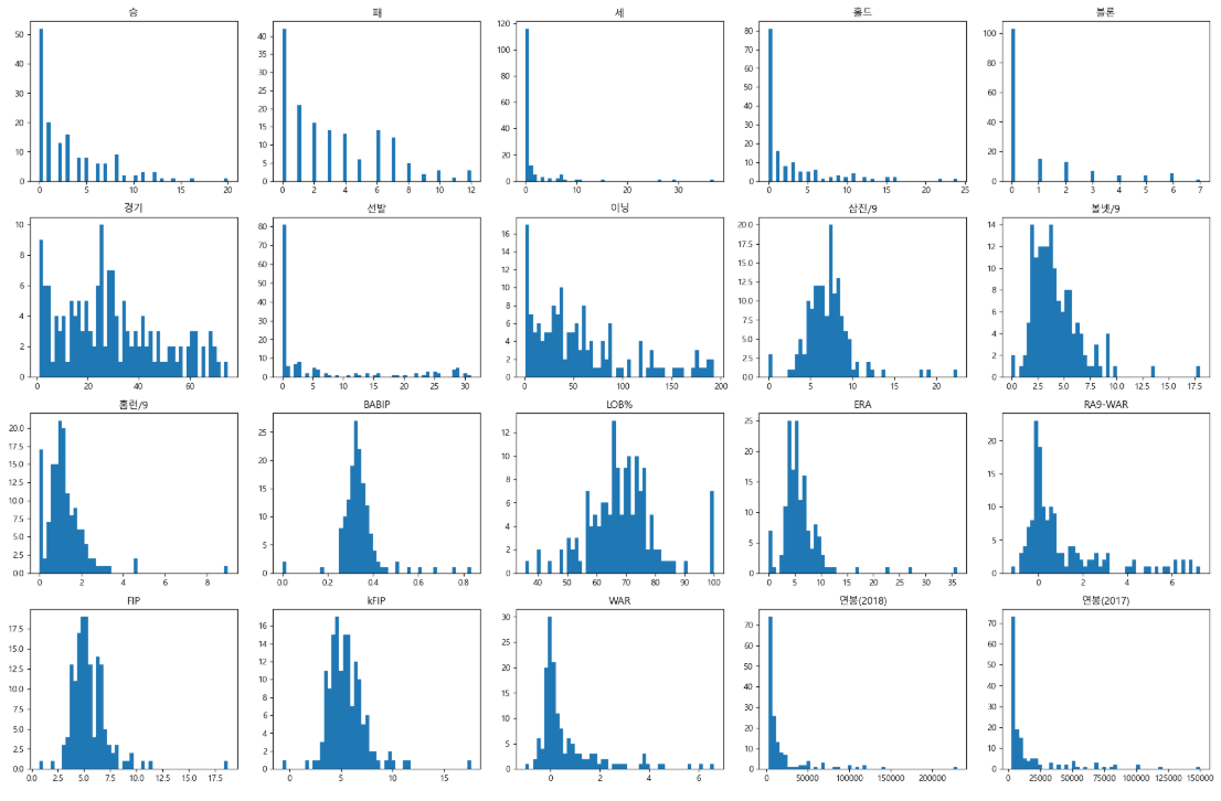
- 매우 불균형한 분포를 가지고 있는 피처들이 많음
- 각 피처간의 단위가 많이 다름
- 스케일링이 필요함
- 선형회귀도 단위가 큰 데이터의 영향을 크게 받을 수 있음
- 스케일링이 필요함
02. 데이터 전처리
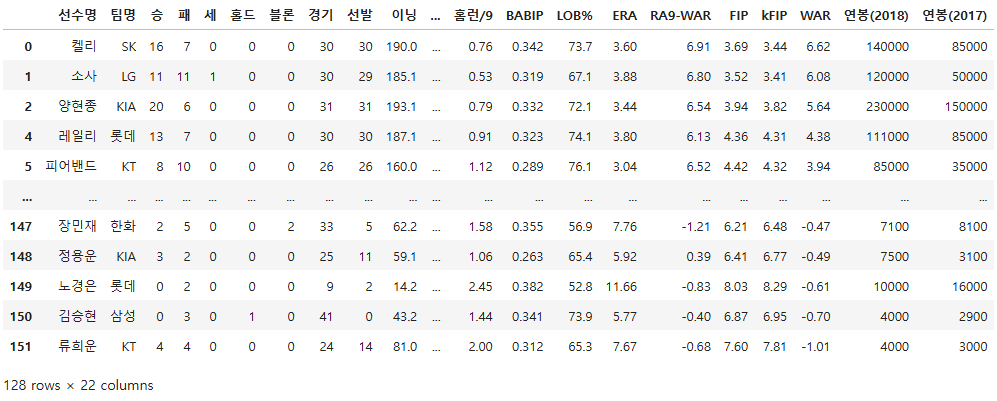
# 재계약하여 연봉이 변화한 선수만 대상으로 필터링
# 재계약을 하지 않는다면 연봉에 변화가 없어 예측이 의미가 없기 때문
pich = pich[pich["연봉(2018)"] != pich["연봉(2017)"]]
pich.shape
(128, 22)
■ 원핫 인코딩
pich["팀명"].unique()
array(['SK', 'LG', 'KIA', '롯데', 'KT', '두산', '삼성', 'NC', '한화'],
      dtype=object)
ohe = OneHotEncoder()
team_arr = np.array(pich["팀명"])
team_arr = np.reshape(team_arr, (-1, 1))
team_name = ohe.fit_transform(team_arr)
ohe.get_feature_names_out()
array(['x0_KIA', 'x0_KT', 'x0_LG', 'x0_NC', 'x0_SK', 'x0_두산', 'x0_롯데',
       'x0_삼성', 'x0_한화'], dtype=object)
team_name
<128x9 sparse matrix of type '<class 'numpy.float64'>'
	with 128 stored elements in Compressed Sparse Row format>
# 원핫인코딩된 데이터를 메모리 효율적으로 나타내기 위해
# sparse matrix(희소행렬) 이라 하고 Compressed Sparse Row를 만듦
# 넘파이 배열로 억지로 변경할 수 있음
team_name.toarray()
array([[0., 0., 0., ..., 0., 0., 0.],
       [0., 0., 1., ..., 0., 0., 0.],
       [1., 0., 0., ..., 0., 0., 0.],
       ...,
       [0., 0., 0., ..., 1., 0., 0.],
       [0., 0., 0., ..., 0., 1., 0.],
       [0., 1., 0., ..., 0., 0., 0.]])
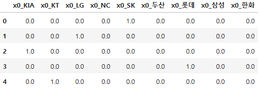
# 데이터 프레임 형태로 나타내면
ohe_team_df = pd.DataFrame(team_name.toarray(), columns = ohe.get_feature_names_out())
ohe_team_df.head()
ohe_team_df.shape
(128, 9)
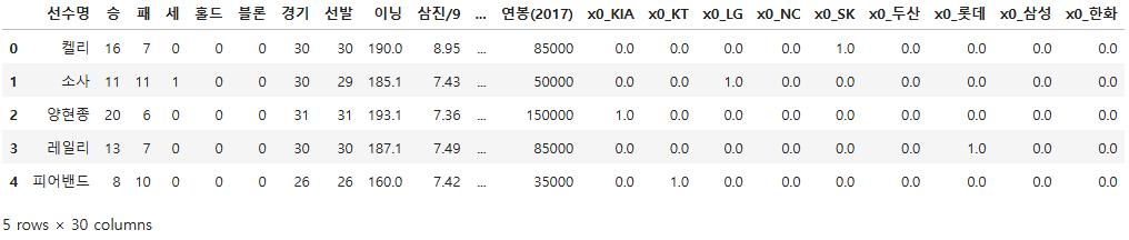
pich.head()
# 인덱스가 다른 데이터 결합을 방지하기 위해 인덱스를 초기화
pich = pd.concat([pich.reset_index(drop = True), ohe_team_df], axis = 1)
pich.shape
(128, 31)
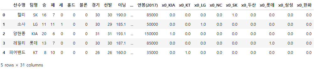
pich.head()
pich = pich.drop("팀명", axis = 1)
pich.head()

pich.shape
(128, 30)
03. 데이터 분할
x = pich.drop(["선수명", "연봉(2018)"], axis = 1)
y = pich["연봉(2018)"]
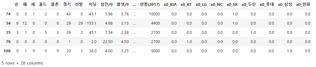
x.head()

x.shape
(128, 28)
x_train, x_test, y_train, y_test = train_test_split(x, y, test_size = 0.2, random_state = 25)
x_train.shape, x_test.shape
((102, 28), (26, 28))
04. 스케일링
x_train.columns
Index(['승', '패', '세', '홀드', '블론', '경기', '선발', '이닝', '삼진/9', '볼넷/9', '홈런/9',
       'BABIP', 'LOB%', 'ERA', 'RA9-WAR', 'FIP', 'kFIP', 'WAR', '연봉(2017)',
       'x0_KIA', 'x0_KT', 'x0_LG', 'x0_NC', 'x0_SK', 'x0_두산', 'x0_롯데', 'x0_삼성',
       'x0_한화'],
      dtype='object')
scale_col = x_train.columns[:-9].tolist()
scale_col
['승',
 '패',
 '세',
 '홀드',
 '블론',
 '경기',
 '선발',
 '이닝',
 '삼진/9',
 '볼넷/9',
 '홈런/9',
 'BABIP',
 'LOB%',
 'ERA',
 'RA9-WAR',
 'FIP',
 'kFIP',
 'WAR',
 '연봉(2017)']
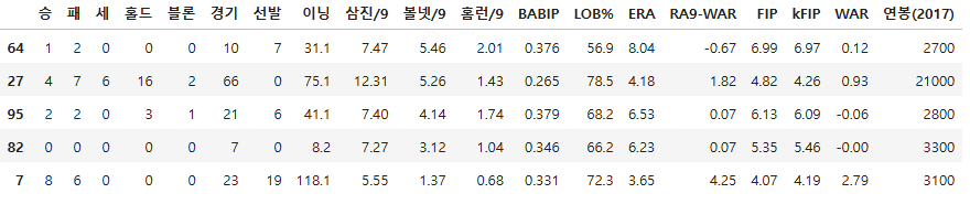
x_train[scale_col].head()
x_train[scale_col].shape
(102, 19)
# StandardScaler: 평균 주변에 몰려있는 정규분포로 몰려있는 성질이 있음 - 선형회귀와의 궁합이 좋은 편
pich_ss = StandardScaler()
scaled_train = pich_ss.fit_transform(x_train[scale_col])
scaled_test = pich_ss.transform(x_test[scale_col])
scaled_test
array([[-8.15155601e-01, -9.90042253e-01,  3.33619898e-02,
        -1.52110180e-01, -5.04497842e-01,  7.79885207e-01,
        -6.39827380e-01, -1.84918927e-01, -4.38035814e-01,
         5.85508690e-01, -4.42443350e-01, -3.35363722e-01,
         6.08132432e-01, -4.18396572e-01, -1.28793008e-01,
        -1.38438820e-01, -4.66625407e-02, -4.24780835e-01,
        -9.88829925e-02],
       [ 8.42237183e-01,  2.89396966e+00, -2.75994643e-01,
        -5.71440945e-01, -5.04497842e-01,  4.86468120e-02,
        ...
scaled_train = pd.DataFrame(scaled_train, columns = scale_col)
scaled_test = pd.DataFrame(scaled_test, columns = scale_col)
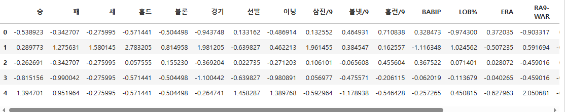
scaled_train.head()
x_train.iloc[:, -9:].head()

scaled_train = pd.concat([scaled_train, x_train.iloc[:, -9:].reset_index(drop = True)], axis = 1)
scaled_test = pd.concat([scaled_test, x_test.iloc[:, -9:].reset_index(drop = True)], axis = 1)
scaled_train.shape, scaled_test.shape
((102, 28), (26, 28))
05. 모델 훈련
lr = LinearRegression()
lr.fit(scaled_train, y_train)
06. 모델 평가
lr.score(scaled_test, y_test)
0.909914311047339
pred = lr.predict(scaled_test)
mae = mean_absolute_error(y_test, pred)
mae
6187.559946438219
07. 모델 최적화
# statsmodels 라이브러리로 회귀 분석
X = sm.add_constant(scaled_train) # 상수항 추가
model = sm.OLS(y_train.reset_index(drop = True), X)
model = model.fit()
model.summary()
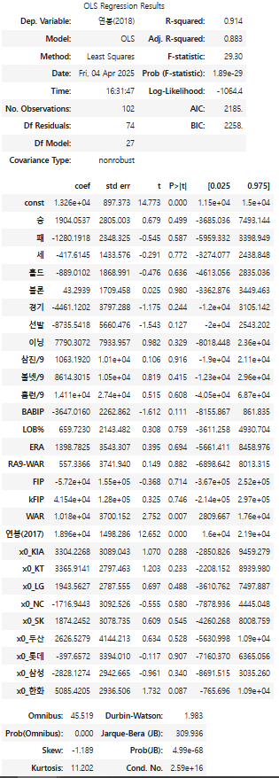
08. 통계적인 지표 보는 법
- F-statistic: 회귀식의 유의성 검정에 사용되는 값으로, Prob(F-statistic)과 함께 해석해야 함
- prob(F-statistic): F통계량에 대한 p-value. 일반적으로 0.05이하면 회귀 분석이 유의미한 의미를 가짐
- p>|t|: 각 피처가 얼마나 유의미한지를 나타내는 p-value
# 계수 시각화
# 회귀 계수를 시리즈로 변환
coefs = model.params.tolist()
coefs_se = pd.Series(coefs)
# 변수명을 리스트로 변환
x_labels = model.params.index.tolist()
model.params
const       13257.168423
승            1904.053672
패           -1280.191750
세            -417.614545
홀드           -889.010204
블론             43.293940
경기          -4461.120243
선발          -8735.541783
이닝           7790.307241
삼진/9         1063.192005
볼넷/9         8614.301539
홈런/9        14105.707516
BABIP       -3647.016049
LOB%          659.723016
ERA          1398.782504
RA9-WAR       557.336602
FIP        -57201.667319
kFIP        41543.808351
WAR         10182.380663
연봉(2017)    18956.003879
x0_KIA       3304.226790
x0_KT        3365.914128
x0_LG        1943.562726
x0_NC       -1716.944325
x0_SK        1874.245240
x0_두산        2626.527859
x0_롯데        -397.657180
x0_삼성       -2828.127354
x0_한화        5085.420540
dtype: float64
ax = coefs_se.plot(kind = "bar")
ax.set_title("feature_coef_graph")
ax.set_xlabel("feature")
ax.set_ylabel("coef")
ax.set_xticklabels(x_labels)
plt.show

# 피처들의 상관관계 시각화
corr = pich[scale_col].corr()
fig = plt.figure(figsize = (20, 20))
hm = sns.heatmap(corr.values, cbar = True, annot = True, square = True, fmt = ".2f",
annot_kws = {"size" : 15}, yticklabels = scale_col, xticklabels = scale_col)
plt.tight_layout()
plt.show()

- 몇몇 피처 쌍에서 높은 연관성을 발견할 수 있음
- 회귀 분석은 피처 간의 독립성을 전제로 하는 분석이기 때문에 올바른 회귀 분석을 하기 위해서는 연관성이 높은 쌍을 제거해야함
- 다중공선성
- 변수 간 상관관계가 높아 분석에 부정적인 영향을 미치는 것
- 모델 성능을 위해 어떤 피처를 제거하는 것이 옳은 판단일지에 대한 기준을 제시할 수 있음
- 다중공선성은 분산팽창요인(Variance Inflation Factor(VIF)) 이라는 계수로 평가
- 일반적으로 VIF가 15를 넘으면 다중 공선성의 문제가 발생했다고 판단함
- 다중공선성
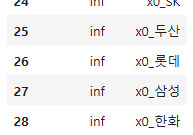
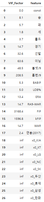
# 피처마다 VIF 계수를 출력
vif = pd.DataFrame()
vif["VIF_Factor"] = [variance_inflation_factor(X.values, i) for i in range(X.shape[1])]
vif["feature"] = X.columns
vif.round(1)
C:\ProgramData\anaconda3\Lib\site-packages\statsmodels\regression\linear_model.py:1783: RuntimeWarning: divide by zero encountered in scalar divide
  return 1 - self.ssr/self.centered_tss
C:\ProgramData\anaconda3\Lib\site-packages\statsmodels\stats\outliers_influence.py:197: RuntimeWarning: divide by zero encountered in scalar divide
  vif = 1. / (1. - r_squared_i)

...
08. 변수 제거
※ 변수 선택법(Variable Selection)
1. 전진 선택법(Forward Selection) : 아무 변수도 포함하지 않은 모델에서 시작하여, 가장 유의미한 변수를 하나씩 추가하는 방법
2. 후진 소거법(Backward Elimination) (*주로 사용*) : 모든 변수가 포함된 모델에서 가장 도움이 되지 않는 변수(p값)를 하나씩 제거하는 방법
3. 단계적 선택법(Stepwise Selection) : 전진 선택법과 후진 제거법을 결합한 방법으로, 변수를 추가하면서 동시에 기존 변수 중 유의미하지 않은 변수를 제거하는 방식. 전진 선택법과 동일하게 시작함.
변수제거 1
- 제거된 변수: 블론
- 무의미한 변수가 다중공선성보다 더 심각한 문제를 유발하기 때문
- 최종적으로는 P값이 높은 변수, VIF가 높은 변수 모두 제거되어야 함
new_X = X.drop("블론", axis = 1)
model = sm.OLS(y_train.reset_index(drop = True), new_X)
model = model.fit()
model.summary()

vif = pd.DataFrame()
vif["VIF_Factor"] = [variance_inflation_factor(new_X.values, i) for i in range(new_X.shape[1])]
vif["feature"] = new_X.columns
vif.round(1)

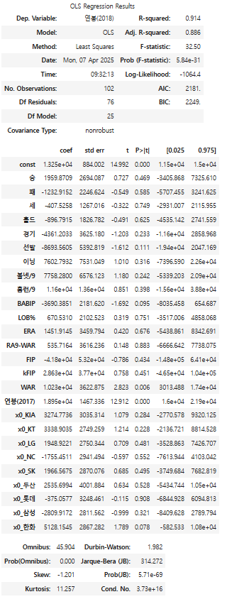
변수제거 2
- 제거된 변수: 블론, 삼진/9
new_X = new_X.drop("삼진/9", axis = 1)
model = sm.OLS(y_train.reset_index(drop = True), new_X)
model = model.fit()
model.summary()
vif = pd.DataFrame()
vif["VIF_Factor"] = [variance_inflation_factor(new_X.values, i) for i in range(new_X.shape[1])]
vif["feature"] = new_X.columns
vif.round(1)
...
# p-value가 0.05보다 높은 값들이 모두 없어질 때 까지 실행(p>|t| 로 판단)
# 모두 없어지지 않더라도 모델 성능이 떨어지면 즉시 중단(AIC, BIC로 판단)
#AIC: 모델적합도, 복합도
#BIC : 모델 복잡도를 크게 설명(낮을수록좋음)
분석결과
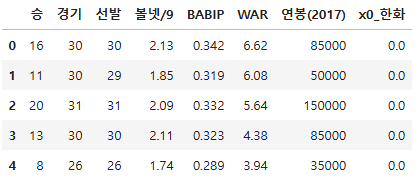
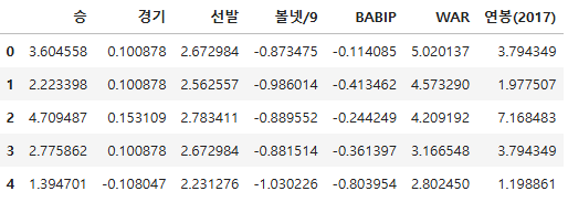
fin_train = scaled_train[["승", "경기", "선발", "볼넷/9", "BABIP", "WAR", "연봉(2017)", "x0_한화"]]
fin_test = scaled_test[["승", "경기", "선발", "볼넷/9", "BABIP", "WAR", "연봉(2017)", "x0_한화"]]
fin_lr = LinearRegression()
fin_lr.fit(fin_train, y_train)
fin_lr.score(fin_test, y_test)
0.9146655001018293
fin_pred = fin_lr.predict(fin_test)
fin_mae = mean_absolute_error(y_test, fin_pred)
fin_mae
5611.38504203962
fin_lr.coef_, fin_lr.intercept_
(array([ 3990.78673446, -3192.58368007, -4545.47447928,  2263.92127989,
        -2604.92368824, 11366.53695719, 18728.62793042,  3761.13489453]),
 14195.748835937602)
fin_train.columns
Index(['승', '경기', '선발', '볼넷/9', 'BABIP', 'WAR', '연봉(2017)', 'x0_한화'], dtype='object')
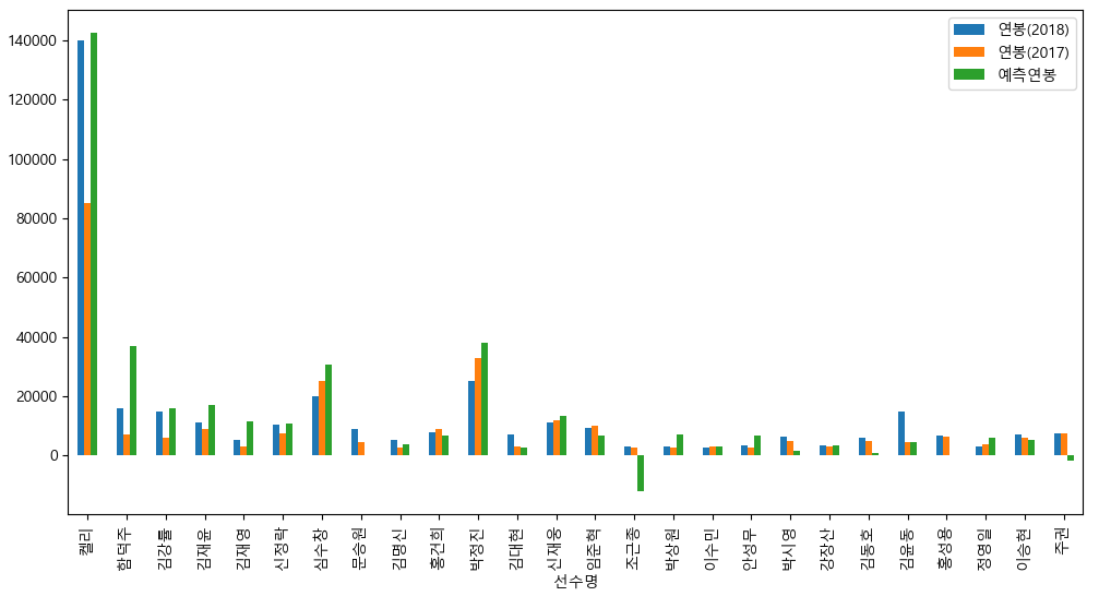
최종 시각화
pich.head()
result_df = pich[fin_train.columns]
result_df.head()
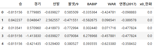
result_df = pich[scale_col]
result_df = pich_ss.transform(result_df)
result_df = pd.DataFrame(result_df, columns = scale_col)
result_df.head()
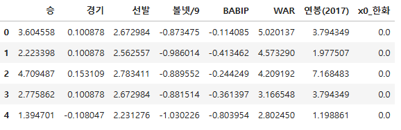
result_df = result_df[['승', '경기', '선발', '볼넷/9', 'BABIP', 'WAR', '연봉(2017)']]
result_df.head()
result_df = pd.concat([result_df, pich["x0_한화"]], axis = 1)
result_df.head()
fin_test.head()
vis_pred = fin_lr.predict(result_df)
vis_pred[:5]
array([142552.94858951,  98961.99663783, 200571.71852621, 118802.93838943,
        64033.50711059])
vis_df = pd.read_csv("./data/picher_stats_2017.csv")
vis_df = vis_df[vis_df["연봉(2018)"] != vis_df["연봉(2017)"]]
vis_df = vis_df.reset_index(drop = True)
vis_df = pd.concat([vis_df, pd.DataFrame(vis_pred, columns = ["예측연봉"])], axis = 1)
vis_df.shape
(128, 23)
vis_df.tail()
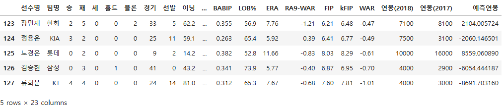
vis_df.head()
x_test.head()
x_test.index
Index([ 74,  34,  35,  79, 108,  40,  87,  41,  83,   6,  20,  26, 116,  54,
        42,  25, 117,  21,  97,   0, 122, 100,  91, 121, 109,  33],
      dtype='int64')
vis_df = vis_df.loc[x_test.index].sort_index()
vis_df.head()

fig = plt.figure(figsize = (12, 6))
vis_df.plot(x = "선수명", y = ["연봉(2018)", "연봉(2017)", "예측연봉"], kind = "bar", ax = plt.gca())
plt.show()
728x90
'08_ML(Machine_Learning)' 카테고리의 다른 글
| 15_로지스틱 감성분류(자연어 처리) - 맛집 리뷰 (6) | 2025.04.08 |
|---|---|
| 14_로지스틱 회귀 (0) | 2025.04.07 |
| 11_Ridge, Lasso, Elastic Net (0) | 2025.04.04 |
| 10_다중 선형 회귀 규제 (0) | 2025.04.04 |
| 09_선형 회귀 실습 (0) | 2025.04.04 |