728x90
선형 회귀 실습
import pandas as pd
import numpy as np
import matplotlib.pyplot as plt
import seaborn as sns
from sklearn.model_selection import train_test_split
from sklearn.linear_model import LinearRegression
from sklearn.metrics import mean_squared_error, root_mean_squared_error
from scipy import stats
01. 데이터 준비
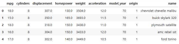
df = pd.read_csv("./data/auto-mpg.csv", header = None)
df.columns = ["mpg", "cylinders", "displacement", "horsepower", "weight", "acceleration", "model_year", "origin", "name"]
df.head()
# 독립변수 cylinders horsepower weight 로 mpg를 예측하는 선형회귀 모델 만들기
df.shape
(398, 9)
df.dtypes
mpg             float64
cylinders         int64
displacement    float64
horsepower       object
weight          float64
acceleration    float64
model_year        int64
origin            int64
name             object
dtype: object
df.describe()

df["horsepower"].unique()
array(['130.0', '165.0', '150.0', '140.0', '198.0', '220.0', '215.0',
       '225.0', '190.0', '170.0', '160.0', '95.00', '97.00', '85.00',
       '88.00', '46.00', '87.00', '90.00', '113.0', '200.0', '210.0',
       '193.0', '?', '100.0', '105.0', '175.0', '153.0', '180.0', '110.0',
       '72.00', '86.00', '70.00', '76.00', '65.00', '69.00', '60.00',
       '80.00', '54.00', '208.0', '155.0', '112.0', '92.00', '145.0',
       '137.0', '158.0', '167.0', '94.00', '107.0', '230.0', '49.00',
       '75.00', '91.00', '122.0', '67.00', '83.00', '78.00', '52.00',
       '61.00', '93.00', '148.0', '129.0', '96.00', '71.00', '98.00',
       '115.0', '53.00', '81.00', '79.00', '120.0', '152.0', '102.0',
       '108.0', '68.00', '58.00', '149.0', '89.00', '63.00', '48.00',
       '66.00', '139.0', '103.0', '125.0', '133.0', '138.0', '135.0',
       '142.0', '77.00', '62.00', '132.0', '84.00', '64.00', '74.00',
       '116.0', '82.00'], dtype=object)
# ?때문에 object형임을 확인했으므로 ?를 제외하고 데이터타입 변경
df = df[df["horsepower"] != "?"]
df.shape
(392, 9)
df["horsepower"] = df["horsepower"].astype(float)
02. 변수 선택
# 분석에 활용할 열 선택(연비, 실린더, 출력, 중량)
ndf = df[["mpg", "cylinders", "horsepower", "weight"]]
ndf.head()

03. 데이터셋 분할
x = ndf.drop("mpg", axis = 1)
y = ndf["mpg"]
x_train, x_test, y_train, y_test = train_test_split(x, y, test_size = 0.3, random_state = 23)
print(x_train.shape, x_test.shape)
(274, 3) (118, 3)
04. 선형 회귀 모델
lr = LinearRegression()
lr.fit(x_train, y_train)

# 결정계수
r_square = lr.score(x_test, y_test)
r_square
0.6533059000280035
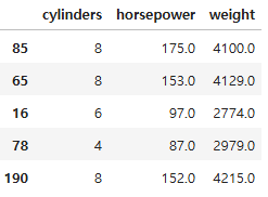
x_train.head()
# 모델 파라미터(모델이 학습한 데이터) 에는 _ 가 붙는다
lr.coef_, lr.intercept_
# y = ax+b
# lr.coef_ : 기울기
# lr.intercept_ : 절편
(array([-0.43494265, -0.04591132, -0.00555456]), 47.47727882907765)
y_pred = lr.predict(x_test)
mse = mean_squared_error(y_test, y_pred)
mse
16.048737054300435
# 굳이 루트를 씌워서 볼 필요가 없으므로(비교만 하면 되므로) mean_squared_error가 개발할 때 더 많이 쓰임
rmse = root_mean_squared_error(y_test, y_pred)
rmse
4.00608749958116
pd.DataFrame({"ans" : y_test, "pred" : y_pred})

05. 모델 평가 시각화
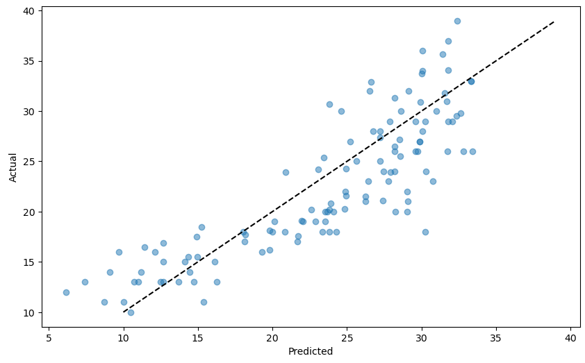
■ 예측값과 정답값 비교 산점도
- 모델의 예측이 실제값과 얼마나 밀접하게 일치하는지 평가
- 완벽한 모델은 모든점이 대각선 위에 놓여 있는 것
plt.figure(figsize = (10, 6))
plt.scatter(y_pred, y_test, alpha = 0.5)
plt.plot([y_test.min(), y_test.max()], [y_test.min(), y_test.max()], "k--")
plt.xlabel("Predicted")
plt.ylabel("Actual")
plt.show()
■ 잔차도
- 잔차의 패턴을 식별하는 데 도움
- 이상적으로는 잔차가 0 주위에 무작위로 흩어져 있어야 하며, 이는 모델의 오류가 무작위임을 나타냄
# 잔차(정답값-예측값)
residuals = y_test - y_pred
residuals
118   -6.307413
328    5.390879
102   -6.794190
276   -3.332704
315   -0.625138
         ...
150   -2.186796
169   -4.090495
316   -2.855628
300    3.030885
19    -7.432965
Name: mpg, Length: 118, dtype: float64
plt.figure(figsize = (10, 6))
plt.scatter(y_pred, residuals, alpha = 0.5) # residuals: 잔차
plt.axhline(y = 0, color = "r", linestyle = "--") # y가 0인 지점에 빨간색 수평선
plt.xlabel("Predicted")
plt.ylabel("Residuals")
plt.show()

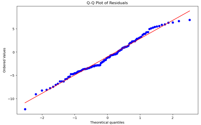
■ QQ plot
- 잔차 분포를 정규 분포와 비교
- 잘 맞는 모델에서는 점들이 대략 대각선을 따라 위치해야 함
plt.figure(figsize = (10, 6))
stats.probplot(residuals.values.flatten(), dist = "norm", plot = plt)
plt.title("Q-Q Plot of Residuals")
plt.show()
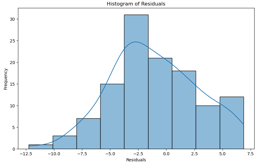
■ 잔차 히스토그램
- 잔차의 분포에 대한 또 다른 시각을 제공
- 잘 맞는 모델의 경우 0을 중심으로 하는 정규 분포를 볼 수 있음
plt.figure(figsize = (10, 6))
sns.histplot(residuals, kde = True)
plt.xlabel("Residuals")
plt.ylabel("Frequency")
plt.title("Histogram of Residuals")
plt.show()
728x90
'08_ML(Machine_Learning)' 카테고리의 다른 글
| 11_Ridge, Lasso, Elastic Net (0) | 2025.04.04 |
|---|---|
| 10_다중 선형 회귀 규제 (0) | 2025.04.04 |
| 08_선형회귀 (0) | 2025.04.04 |
| 07_KNN구현(Numpy(넘파이)) (0) | 2025.04.04 |
| 06_KNN 심화 (0) | 2025.04.04 |