728x90
KNN 심화
# Anaconda Prompt에서 pip install mglearn 로 mglearn 설치
import mglearn
import matplotlib.pyplot as plt
import pandas as pd
from sklearn.preprocessing import MinMaxScaler
from sklearn.model_selection import train_test_split
from sklearn.neighbors import KNeighborsClassifier
from sklearn.decomposition import PCA
from matplotlib.colors import ListedColormap
import warnings #경고메세지 없애주는 코드
warnings.filterwarnings("ignore")
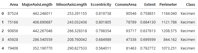
df = pd.read_excel("./data/Raisin_Dataset.xlsx")
df.head()
# 독립변수와 종속변수 분리
x = df.drop(["Area", "Class"], axis = 1)
y = df[["Class"]]
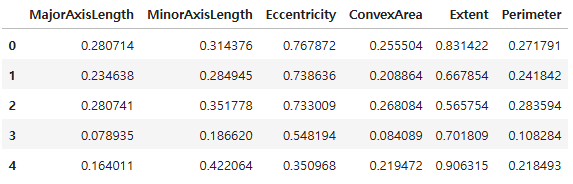
# 독립변수 데이터 정규화 적용
mm = MinMaxScaler()
df_minmax = mm.fit_transform(x)
x = pd.DataFrame(df_minmax, columns = x.columns)
x.head()
# train/test split(7 : 3)
x_train, x_test, y_train, y_test = train_test_split(x, y, test_size = 0.3, stratify = y, random_state = 23)
print(x_train.shape, x_test.shape)
(630, 6) (270, 6)
- KNN 모델은 거리 기반으로 분류를 하기 때문에 독립변수의 스케일을 정규화
- 7 : 3의 비율로 학습셋과 테스트셋을 분리
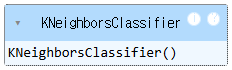
# 기본 KNN 모델 생성 및 적용
knn = KNeighborsClassifier(n_neighbors = 5,
weights = "uniform",
metric = "minkowski")
knn.fit(x_train, y_train)
# KNN 모델 정확도
print(knn.score(x_train, y_train))
print(knn.score(x_test, y_test))
0.8857142857142857
0.8629629629629629
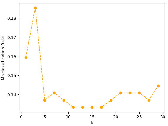
# 이웃 k 수 1 ~ 30 엘보우차트 시각화(거리 가중치 미적용)
# k 범위 지정
k_num = range(1, 31, 2)
accuracies = []
for k in k_num:
k_num_model_1 = KNeighborsClassifier(n_neighbors = k, weights = "uniform")
k_num_model_1. fit(x_train, y_train)
accuracies.append(1 - k_num_model_1.score(x_test, y_test))
plt.plot(k_num, accuracies, "o--", color = "orange")
plt.xlabel("k")
plt.ylabel("Misclassification Rate")
plt.show()
accuracies
[0.1592592592592592,
 0.18518518518518523,
 0.13703703703703707,
 0.14074074074074072,
 0.13703703703703707,
 0.1333333333333333,
 0.1333333333333333,
 0.1333333333333333,
 0.1333333333333333,
 0.13703703703703707,
 0.14074074074074072,
 0.14074074074074072,
 0.14074074074074072,
 0.13703703703703707,
 0.1444444444444445]
- 거리 가중치를 적용하지 않은 모델에서 k 이웃 수를 1에서 30까지 늘려가며 KNN모델의 오분류율을 시각화
- 이웃 수가 11개일 때 오분류율이 가장 낮아져서 k는 11일 때 가장 적합함
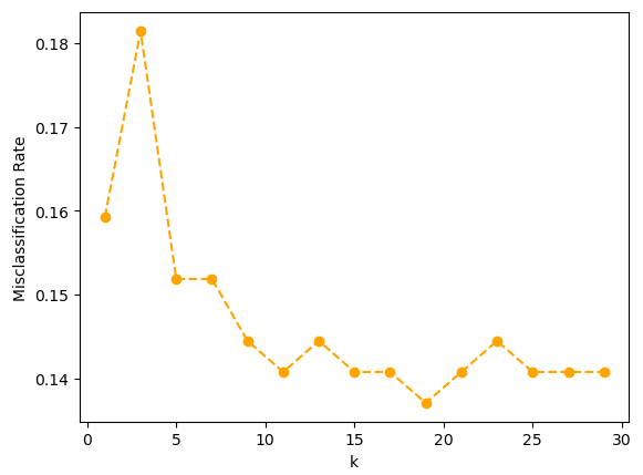
# 이웃 k 수 1 ~ 30까지 엘보우차트 시각화(거리 가중치 적용)
# k 범위 지정
k_num = range(1, 31, 2)
accuracies = []
for k in k_num:
k_num_model_2 = KNeighborsClassifier(n_neighbors = k, weights = "distance")
k_num_model_2. fit(x_train, y_train)
accuracies.append(1 - k_num_model_2.score(x_test, y_test))
plt.plot(k_num, accuracies, "o--", color = "orange")
plt.xlabel("k")
plt.ylabel("Misclassification Rate")
plt.show()
accuracies
[0.1592592592592592,
 0.18148148148148147,
 0.1518518518518519,
 0.1518518518518519,
 0.1444444444444445,
 0.14074074074074072,
 0.1444444444444445,
 0.14074074074074072,
 0.14074074074074072,
 0.13703703703703707,
 0.14074074074074072,
 0.1444444444444445,
 0.14074074074074072,
 0.14074074074074072,
 0.14074074074074072]
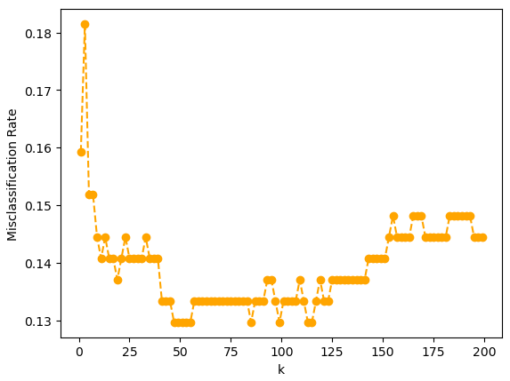
# 이웃 k 수 1 ~ 200까지 엘보우차트 시각화(거리 가중치 적용)
# k 범위 지정
k_num = range(1, 200, 2)
accuracies = []
for k in k_num:
k_num_model_2 = KNeighborsClassifier(n_neighbors = k, weights = "distance")
k_num_model_2. fit(x_train, y_train)
accuracies.append(1 - k_num_model_2.score(x_test, y_test))
plt.plot(k_num, accuracies, "o--", color = "orange")
plt.xlabel("k")
plt.ylabel("Misclassification Rate")
plt.show()
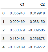
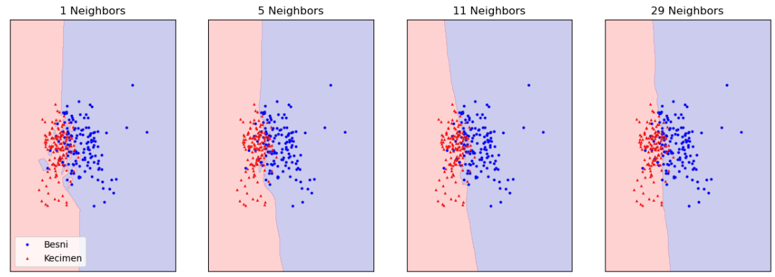
# 시각화를 위한 차원 축소(6차원 -> 2차원)
# 주성분 개수 설정(2개)
pca = PCA(n_components = 2)
df_pca = pca.fit_transform(x_test)
df_pca = pd.DataFrame(df_pca, columns = ["C1", "C2"])
df_pca.head()
# 결정 경계선(decision boundary) 시각화 확인
df_vsl_x = df_pca.to_numpy()
df_vsl_y = y_test["Class"].to_numpy()
# 그래프 설정
cmap_bold = ListedColormap(["#FF0000", "#00FF00"])
fig, axes = plt.subplots(1, 4, figsize = (15, 5))
# 이웃 수 1, 5, 11, 29 에 따른 결정 경계 시각화
for n_neighbors, ax in zip([1, 5, 11, 29], axes):
# k_num_model_eg = KNeighborsClassifier(n_neighbors = n_neighbors)
# k_num_model_eg.fit(df_pca, y_test)
k_num_model_eg = KNeighborsClassifier(n_neighbors = n_neighbors).fit(df_vsl_x, df_vsl_y)
mglearn.plots.plot_2d_separator(k_num_model_eg, df_vsl_x, fill = True, eps = 0.5, ax = ax, alpha = 0.2)
# mglearn.discrete_scatter(df_pca.iloc[:, 0], df_pca.iloc[:, 1], y_test["Class"],
# markeredgewidth = 0.1, c = ["b", "r"], s = 3, ax = ax)
mglearn.discrete_scatter(df_vsl_x[:, 0], df_vsl_x[:, 1], df_vsl_y,
markeredgewidth = 0.1, c = ["b", "r"], s = 3, ax = ax)
ax.set_title(f"{n_neighbors} Neighbors")
axes[0].legend(loc = 3)
plt.show()
# 거리 가중치 추가(weights = "distance")
fig, axes = plt.subplots(1, 4, figsize = (15, 5))
# 이웃 수 1, 5, 11, 29 에 따른 결정 경계 시각화
for n_neighbors, ax in zip([1, 5, 11, 29], axes):
k_num_model_eg = KNeighborsClassifier(n_neighbors = n_neighbors, weights = "distance").fit(df_vsl_x, df_vsl_y)
mglearn.plots.plot_2d_separator(k_num_model_eg, df_vsl_x, fill = True, eps = 0.5, ax = ax, alpha = 0.2)
mglearn.discrete_scatter(df_vsl_x[:, 0], df_vsl_x[:, 1], df_vsl_y,
markeredgewidth = 0.1, c = ["b", "r"], s = 3, ax = ax)
ax.set_title(f"{n_neighbors} Neighbors")
axes[0].legend(loc = 3)
plt.show()

728x90
'08_ML(Machine_Learning)' 카테고리의 다른 글
| 08_선형회귀 (0) | 2025.04.04 |
|---|---|
| 07_KNN구현(Numpy(넘파이)) (0) | 2025.04.04 |
| 05_KNN회귀 (0) | 2025.04.04 |
| 04_KNN_타이타닉 분류 (0) | 2025.04.02 |
| 03_데이터 전처리 (0) | 2025.04.02 |