728x90
주 성분 분석
차원 축소
- 과일 사진의 경우는 10000개의 픽셀이 있기 때문에 10000개의 특성이 있음
- 차원의 저주
- 일반적인 머신러닝 문제는 수천~수백만 개의 특성을 가지고 있는 경우도 있음
- 특성이 너무 많으면 훈련이 느리게 될 뿐 아니라 좋은 솔루션을 찾기 어렵게 됨
- 이러한 문제를 차원의 저주(curse of dimensionality)라고 함
- 차원 축소(dimensionality reduction)
- 데이터를 가장 잘 나타내는 일부 특성을 선택하여 데이터 크기를 줄이고 모델의 성능을 향상시키는 방법
- 예) 이미지 경계면의 배경 부분 제거, 서로 인접한 픽셀들을 결합 등
- 데이터를 가장 잘 나타내는 일부 특성을 선택하여 데이터 크기를 줄이고 모델의 성능을 향상시키는 방법
주성분 분석(principal component analysis)
- 데이터에 있는 분산이 큰 방향을 찾는 것
- 분산: 데이터가 퍼져 있는 정도
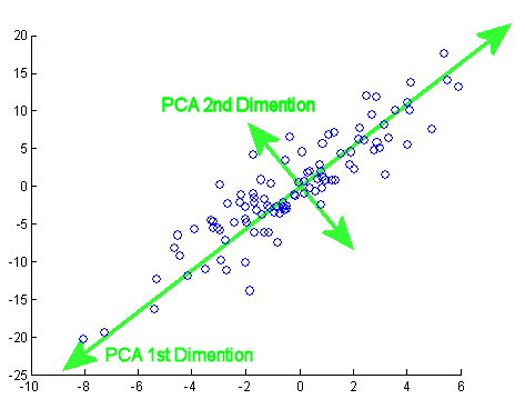
- 위 그림의 데이터에서는 오른쪽 위를 향하는 분산이 가장 큼
- 원본 데이터를 가장 잘 설명하는 방향이 주성분(principal component)
- 주성분은 데이터가 가진 특성을 가장 잘 나타내기 때문에 주성분에 데이터를 투영하면 정보의 손실을 줄이면서 차원을 축소할 수 있음

import numpy as np
import matplotlib.pyplot as plt
from sklearn.decomposition import PCA
from sklearn.linear_model import LogisticRegression
from sklearn.model_selection import cross_validate
from sklearn.cluster import KMeans
fruits = np.load("./data/fruits_300.npy")
fruits.shape
(300, 100, 100)
fruits_2d = fruits.reshape(-1, 100 * 100)
fruits_2d.shape
(300, 10000)
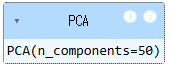
pca = PCA(n_components = 50) # n_components: 주 성분의 개수(임의지정)
pca.fit(fruits_2d)
# pca가 찾은 주성분 확인
pca.components_.shape
(50, 10000)
# 각 클러스터가 어떤 데이터를 나타내는지 출력하는 함수
def draw_fruits(arr):
n = len(arr) # 샘플 수
# 한 줄에 10개씩 이미지를 그릴 때, 몇 개 행이 필요할지 행 개수 계산
rows = int(np.ceil(n / 10))
cols = 10
fig, axs = plt.subplots(rows, cols, figsize = (cols, rows), squeeze = False)
for i in range(rows):
for j in range(cols):
if i * 10 + j < n:
axs[i, j].imshow(arr[i * 10 + j], cmap = "gray_r")
axs[i, j].axis("off")
plt.show()
draw_fruits(pca.components_.reshape(-1, 100, 100))
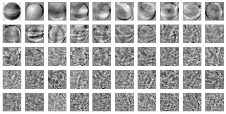
- 주성분은 원본 데이터에서 가장 분산이 큰 방향을 순서대로 나타냄
- 데이터셋에 있는 특징을 찾아낸 것
fruits_2d.shape
(300, 10000)
# 원본 데이터의 차원을 50차원으로 축소
fruits_pca = pca.transform(fruits_2d)
fruits_pca.shape
(300, 50)
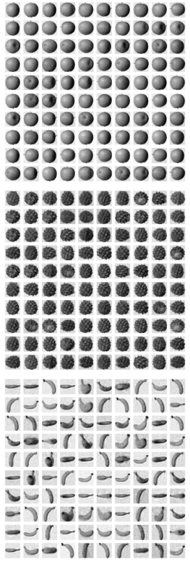
원본 데이터 재구성
- 10000개의 특성을 50개로 줄이면 정보 손실이 없을 수 없지만 정보 손실을 최소한으로 했기 때문에 축소된 데이터에 가깝게 복구 할 수 있음
fruits_inverse = pca.inverse_transform(fruits_pca)
print(fruits_inverse.shape)
(300, 10000)
fruits_reconstruct = fruits_inverse.reshape(-1, 100, 100)
for start in [0, 100, 200]:
draw_fruits(fruits_reconstruct[start: start + 100])
print()
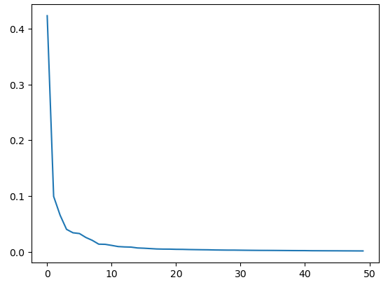
설명된 분산(explained variance)
- 주 성분이 원본 데이터의 분산을 얼마나 잘 나타내는지 기록한 값
- pca클래스의 explained_variance_ratio_ 에 설명된 분산 비율이 기록되어 있음
# 50개의 주성분으로 표현하고 있는 총 분산 비율
print(np.sum(pca.explained_variance_ratio_))
0.9214864344805443
pca.explained_variance_ratio_
array([0.42357017, 0.09941755, 0.06577863, 0.04031172, 0.03416875,
       0.03281329, 0.02573267, 0.02054963, 0.01372276, 0.01342773,
       0.01152146, 0.00944596, 0.00878232, 0.00846697, 0.00693049,
       0.00645188, 0.00578896, 0.00511202, 0.00486383, 0.00480347,
       0.00447832, 0.00437315, 0.0040804 , 0.00389473, 0.00372441,
       0.00359286, 0.00331467, 0.0031784 , 0.00304329, 0.00303757,
       0.00288909, 0.00275657, 0.00264878, 0.00255885, 0.0025216 ,
       0.00247208, 0.00239315, 0.00230835, 0.00222117, 0.00216417,
       0.00213877, 0.00196738, 0.0019274 , 0.00187715, 0.00183741,
       0.00180512, 0.00172993, 0.00169104, 0.00162324, 0.00157714])
plt.plot(pca.explained_variance_ratio_)
plt.show()
설명된 분산의 비율로 pca사용
pca = PCA(n_components = 0.75)
pca.fit(fruits_2d)

pca.n_components_
9
print(np.sum(pca.explained_variance_ratio_))
0.756065165999834
# 설명된 분산의 50%에 달하는 주성분을 찾도록 설정
pca = PCA(n_components = 0.5)
pca.fit(fruits_2d)
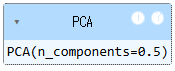
# 2개의 특성만으로도 원본 데이터 분산의 50%를 표현할 수 있음
pca.n_components_
2
print(np.sum(pca.explained_variance_ratio_))
0.52298772458006
다른 알고리즘과 함께 사용하기
# 레이블 생성
# 사과 = 0, 파인애플 = 1, 바나나 = 2
y = np.array([0] * 100 + [1] * 100 + [2] * 100)
lr = LogisticRegression()
# 원본 데이터로 성능 테스트
scores = cross_validate(lr, fruits_2d, y)
print(np.mean(scores["test_score"]))
print(np.mean(scores["fit_time"]))
0.9966666666666667
0.1445704936981201
# pca로 50개의 주성분으로 축소한 데이터로 성능 테스트
scores = cross_validate(lr, fruits_pca, y)
print(np.mean(scores["test_score"]))
print(np.mean(scores["fit_time"]))
0.9966666666666667
0.005481576919555664
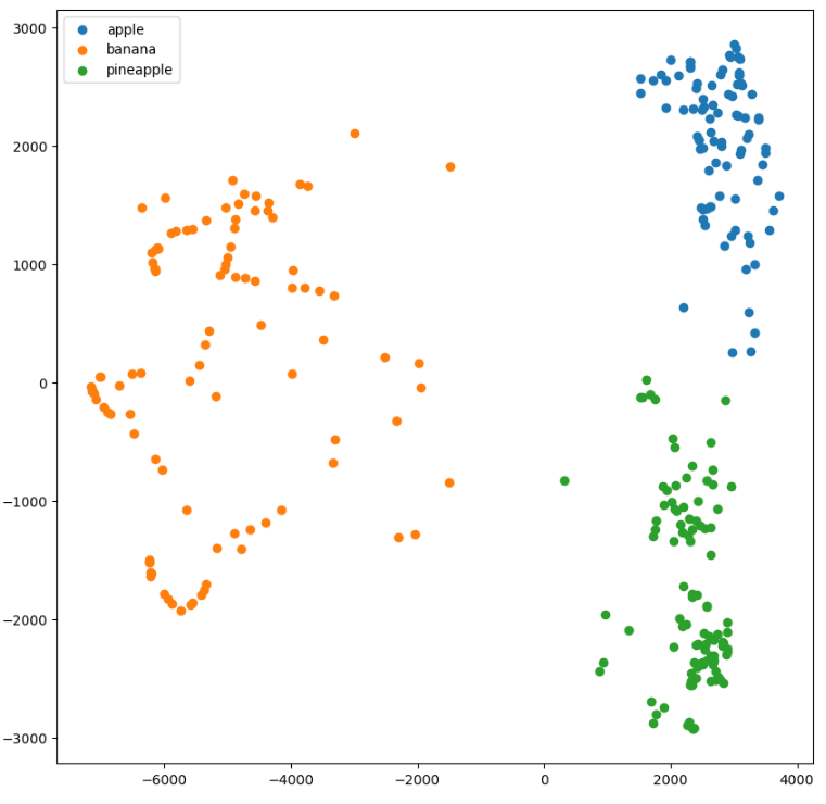
차원 축소된 데이터로 kmeans 사용
pca.n_components_
2
# 2개의 주성분으로 차원 축소
fruits_pca = pca.transform(fruits_2d)
print(fruits_pca.shape)
(300, 2)
km = KMeans(n_clusters = 3, random_state = 26)
km.fit(fruits_pca)
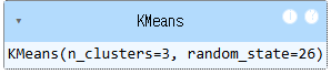
print(np.unique(km.labels_, return_counts = True))
(array([0, 1, 2]), array([ 91, 99, 110], dtype=int64))
차원 축소된 데이터로 시각화
plt.figure(figsize = (10, 10))
for label in range(3):
data = fruits_pca[km.labels_ == label]
plt.scatter(data[:, 0], data[:, 1])
plt.legend(["apple", "banana", "pineapple"])
plt.show()
'08_ML(Machine_Learning)' 카테고리의 다른 글
| scikit-learn algorithm cheat sheet(사이킷런 알고리즘 치트시트) (0) | 2025.04.14 |
|---|---|
| 29_군집분석_연습문제 (0) | 2025.04.14 |
| 27_군집모델_심화 (2) | 2025.04.11 |
| 26_군집 알고리즘(k-means) (0) | 2025.04.11 |
| 25_군집 알고리즘(비지도 학습)-과일 사진 레이블 없이 분류 (0) | 2025.04.11 |