728x90
모델링 전략
- 베이스라인 모델 : 가장 기본적인 선형회귀 모델
- 타깃값은 log(count) 사용
데이터 전처리
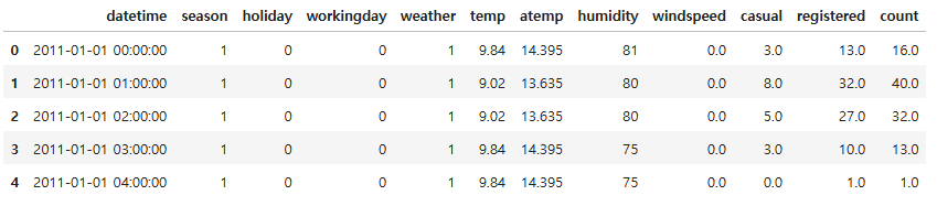
train_df = pd.read_csv("./data/bike/train.csv")
test_df = pd.read_csv("./data/bike/test.csv")
submission_df = pd.read_csv("./data/bike/sampleSubmission.csv")
train_df = train_df[train_df["weather"] != 4]
train_df.shape, test_df.shape
# train데이터와 test데이터를 합쳐서 전처리 후
# 종속변수가 null인 데이터와 아닌 데이터로 나누면 다시 train과 test로 나누어짐
all_df = pd.concat([train_df, test_df], ignore_index = True)
all_df.head()
all_df.tail()

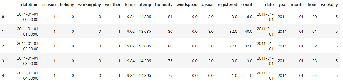
all_df["date"] = all_df["datetime"].map(lambda x: x.split()[0])
all_df["year"] = all_df["datetime"].map(lambda x: x.split()[0].split("-")[0])
all_df["month"] = all_df["datetime"].map(lambda x: x.split()[0].split("-")[1])
all_df["hour"] = all_df["datetime"].map(lambda x: x.split()[1].split(":")[0])
all_df["weekday"] = all_df["date"].map(lambda x: pd.to_datetime(x).weekday())
all_df.head()
변수제거
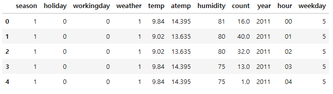
drop_features = ["casual", "registered", "datetime", "date", "month", "windspeed"]
all_df = all_df.drop(drop_features, axis = 1)
all_df.head()
데이터 분할
# ~ 은 not을 의미
train = all_df[~pd.isna(all_df["count"])]
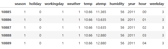
test = all_df[pd.isna(all_df["count"])]
train.shape, test.shape
((10885, 11), (6493, 11))
x_train = train.drop("count", axis = 1)
x_test = test.drop("count", axis = 1)
y = train["count"]
x_train.shape, x_test.shape, y.shape
((10885, 10), (6493, 10), (10885,))
x_train.head()

x_test.head()
베이스라인 모델
log_y = np.log(y)
rmsle_scorer = make_scorer(rmsle, greater_is_better = False)
lr_l = LinearRegression()
lr_l.fit(x_train, log_y)

lr_n = LinearRegression()
lr_n.fit(x_train, y)

pred_l = lr_l.predict(x_train)
pred_n = lr_n.predict(x_train)
# 예측값과 정답값 비교
print(rmsle(log_y, pred_l, True))
print(rmsle(y, pred_n, False))
1.0204980189305024
1.2936714652321617
- log(count)로 예측한 모델이 더 성능이 좋은 것을 확인
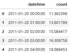
pred = lr_l.predict(x_test)
# 지수 변환으로 로그 씌우기 전 상태로 복구
pred = np.exp(pred)
pred
array([ 11.36239802,  13.60178871,  15.084417  , ..., 140.11446305,
       169.34534711, 163.86682443])
submission_df["count"] = pred
submission_df.head()
submission_df.to_csv("submission_test.csv", index = False)
릿지
rid = Ridge(random_state = 26)
# 하이퍼파라미터 값 목록
ridge_params = {"alpha" : [0.1, 1, 2, 3, 4, 10, 30, 100, 200]}
# 분할기(train_test_split을 안 했으므로, 데이터 섞기)
splitter = KFold(n_splits = 5, shuffle = True, random_state = 26)
rmsle_scorer = make_scorer(rmsle, greater_is_better = False)
# 그리드서치 객체 생성
gs_rid = GridSearchCV(estimator = rid, # 릿지 모델
param_grid = ridge_params, # 값 목록
scoring = rmsle_scorer, # 평가지표
cv = splitter) # 교차검증 분할 수
gs_rid.fit(x_train, log_y)

gs_rid.best_params_
{'alpha': 100}
gs_rid.cv_results_["mean_test_score"]
array([-1.02166885, -1.02166744, -1.02166589, -1.02166435, -1.02166285,
       -1.02165425, -1.02163063, -1.02159467, -1.0216318 ])
gs_rid.best_score_
-1.0215946748914564
preds = gs_rid.predict(x_test)
preds = np.exp(preds)
submission_df["count"] = preds
submission_df.to_csv("submission_test_rid.csv", index = False)
- 1.02109
# 릿지 하이퍼파라미터로 성능이 약간 더 좋아짐
라쏘
las = Lasso(random_state = 26)
# 하이퍼파라미터 값 목록
lasso_alpha = 1 / np.array([0.1, 1, 2, 3, 4, 10, 30, 100, 200])
lasso_params = {"alpha" : lasso_alpha}
# 그리드서치 객체 생성
gs_las = GridSearchCV(estimator = las,
param_grid = lasso_params,
scoring = rmsle_scorer,
cv = splitter)
gs_las.fit(x_train, log_y)
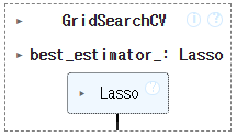
gs_las.best_params_
{'alpha': 0.005}
gs_las.best_score_
-1.021239955263354
preds = gs_las.predict(x_test)
preds = np.exp(preds)
submission_df["count"] = preds
submission_df.to_csv("submission_test_las.csv", index = False)
- 1.0206
랜덤포레스트
rf = RandomForestRegressor(random_state = 26)
# 그리드서치 객체 생성
rf_params = {"n_estimators" : [100, 120, 140, 160]}
gs_rf = GridSearchCV(estimator = rf,
param_grid = rf_params,
scoring = rmsle_scorer,
cv = splitter)
gs_rf.fit(x_train, log_y)
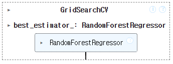
gs_rf.best_params_
{'n_estimators': 160}
gs_rf.best_score_
-0.31040227116204316
preds = gs_rf.predict(x_test)
preds = np.exp(preds)
submission_df["count"] = preds
submission_df.to_csv("submission_test_rf.csv", index = False)
- 0.39531
gs_rf.best_estimator_.feature_importances_
array([0.03648298, 0.00160072, 0.03928598, 0.0117874 , 0.04932995,
       0.01942053, 0.02320008, 0.03187894, 0.7571596 , 0.02985382])
x_train.columns
Index(['season', 'holiday', 'workingday', 'weather', 'temp', 'atemp',
       'humidity', 'year', 'hour', 'weekday'],
      dtype='object')
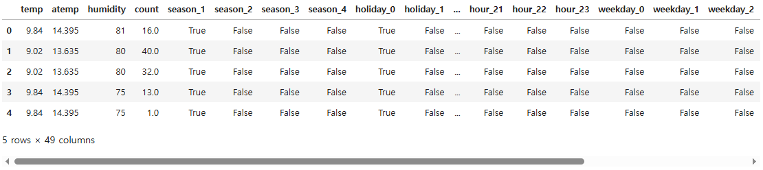
# 원핫인코딩
# 공휴일 등 범주형 데이터를 원핫인코딩
all_ohe = pd.get_dummies(all_df, columns = ["season", "holiday", "workingday", "weather", "year",
"hour", "weekday"])
all_ohe.head()
train_ohe = all_ohe[~pd.isna(all_df["count"])]
test_ohe = all_ohe[pd.isna(all_df["count"])]
x_train_ohe = train_ohe.drop("count", axis = 1)
x_test_ohe = test_ohe.drop("count", axis = 1)
선형회귀 + 원핫인코딩
lr_ohe = LinearRegression()
lr_ohe.fit(x_train_ohe, log_y)
preds = lr_ohe.predict(x_train_ohe)
rmsle(log_y, preds, True)
0.582961267259857
랜덤포레스트 + 원핫인코딩
rf = RandomForestRegressor(random_state = 26)
gs_rf = GridSearchCV(estimator = rf,
param_grid = rf_params,
scoring = rmsle_scorer,
cv = splitter)
gs_rf.fit(x_train_ohe, log_y)

preds = gs_rf.predict(x_test_ohe)
preds = np.exp(preds)
submission_df["count"] = preds
submission_df.to_csv("submission_test_rf_ohe.csv", index = False)
- 0.40448
'08_ML(Machine_Learning)' 카테고리의 다른 글
| 32_자전거 대여 수요 예측(1) (1) | 2025.04.17 |
|---|---|
| 31_피마인디언 당뇨병 예측 (0) | 2025.04.16 |
| 30_머신러닝 프로젝트 프로세스(머신러닝 모델링 프로세스) (0) | 2025.04.15 |
| scikit-learn algorithm cheat sheet(사이킷런 알고리즘 치트시트) (0) | 2025.04.14 |
| 29_군집분석_연습문제 (0) | 2025.04.14 |