13_T-Test

T-Test

 

from scipy import stats
import pandas as pd
import seaborn as sns
import matplotlib.pyplot as plt

df = pd.read_csv("./data/Golf_test.csv")

df.head()

 

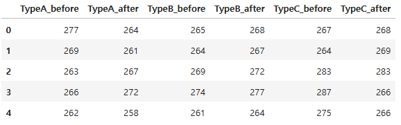
• A, B, C 세 개 타입의 골프공의 비거리 테스트 결과 데이터
• 각 타입의 골프공을 특정 처리를 하기 전과 후로 구분

 

df.shape

(50, 6)

 

df.dtypes

TypeA_before    int64
TypeA_after     int64
TypeB_before    int64
TypeB_after     int64
TypeC_before    int64
TypeC_after     int64
dtype: object

 

df.info()

<class 'pandas.core.frame.DataFrame'>
RangeIndex: 50 entries, 0 to 49
Data columns (total 6 columns):
 #   Column        Non-Null Count  Dtype
---  ------        --------------  -----
 0   TypeA_before  50 non-null     int64
 1   TypeA_after   50 non-null     int64
 2   TypeB_before  50 non-null     int64
 3   TypeB_after   50 non-null     int64
 4   TypeC_before  50 non-null     int64
 5   TypeC_after   50 non-null     int64
dtypes: int64(6)
memory usage: 2.5 KB

 

df.describe()

 

• 평균값은 270 내외의 값을 가지고 있으며, before 보다 after가 큰 경향이 있음
• B, C, A 순으로 평균값이 큼
• 비거리 평균의 차이가 통계적으로 유의미한 차이인지 확인

# 그룹별 박스 플롯 시각화
df2 = pd.melt(df)
df2.head()

 

 

 

df2.shape

(300, 2)

 

plt.figure(figsize = (12, 6))
sns.boxplot(x = "variable", y = "value", data = df2)
plt.title("Golf ball test")
plt.show()

 

• 컬럼별 차이를 직관적으로 확인하기 위해 시각화
• TypeA_before 와 TypeA_after는 중앙값은 차이가 나지만 분포는 유사함

# 데이터 정규성 검정
print(stats.shapiro(df["TypeA_before"]))
print(stats.shapiro(df["TypeA_after"]))
print(stats.shapiro(df["TypeB_before"]))
print(stats.shapiro(df["TypeB_after"]))
print(stats.shapiro(df["TypeC_before"]))
print(stats.shapiro(df["TypeC_after"]))

ShapiroResult(statistic=0.9655377158052212, pvalue=0.15154941346876938)
ShapiroResult(statistic=0.9728279567361319, pvalue=0.30051020169283893)
ShapiroResult(statistic=0.9730037974106026, pvalue=0.305345354286895)
ShapiroResult(statistic=0.9693011028933032, pvalue=0.2167560294629035)
ShapiroResult(statistic=0.9595516780117022, pvalue=0.08512947305030288)
ShapiroResult(statistic=0.946983211173158, pvalue=0.02568194780152731)

• pvalue 값이 0.05를 초과하면 정규성을 만족
• pvalue 값이 0.05를 초과하지 않으면 정규성을 만족하지 않음
  • TypeC_after는 정규성을 가지지 못하기 때문에 이상치 처리나 스케일링 등을 적용하여 정규성을 갖도록 가공해야함

# 데이터 등분산성 검정
stats.bartlett(df["TypeA_before"], df["TypeA_after"],
               df["TypeB_before"], df["TypeB_after"])

BartlettResult(statistic=1.5469416874551807, pvalue=0.6714793492170279)

 

 

• pvalue가 0.05를 초과하면 등분산성을 만족

# 대응표본 t검정 수행
stats.ttest_rel(df["TypeA_before"], df["TypeA_after"])

TtestResult(statistic=-1.221439914972903, pvalue=0.227763764486876, df=49)

 

• pvalue 가 0.05를 초과하여 평균의 차이가 통계적으로 유의미하지 않음
  • 즉, TypeA 골프공은 특정 처리를 하기 전과 후의 비거리가 통계적으로 차이가 없음

stats.ttest_rel(df["TypeB_before"], df["TypeB_after"])

TtestResult(statistic=-34.99999999999999, pvalue=2.4886054257756526e-36, df=49)

 

# TypeB 골프공은 pvalue가 0.05이하이므로 통계적으로 유의미

# p - value > 0.05 -> H0 채택
# p - value <= 0.05 -> H0 기각 -> H1 채택

 

# 독립표본 t검정 수행
stats.ttest_ind(df["TypeA_before"], df["TypeB_before"], equal_var = True) #등분산성:equal_var = True입력

TtestResult(statistic=-2.7894959746581156, pvalue=0.00634384977076247, df=98.0)

 

• pvalue가 0.05보다 작아 A와 B 두 집단간에는 통계적으로 유의미한 차이가 있음

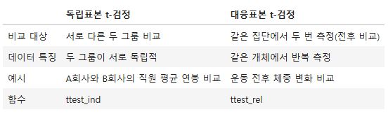
• 대응표본 t검정과 독립표본 t검정의 차이